Optimization modeling tools and parser solvers, such as CVXPY, make solving deterministic optimization problems a lot easier: they allow users to encode optimization problems in high-level mathematical expressions thereby reducing the need for tedious reformulations or fitting problems into canonical forms.
Many optimization problems often include uncertain terms which are modeled as random variables. Examples of such random variables include stock returns, sensor readings, or the state of a system (e.g. localization of a robot which is uncertain). This gives rise to Risk-Based Optimization problems.
Risk-based optimization problems can be hard to code and they may require tedious reformulations or digging up equivalent forms to eventually encode the problem as an equivalent deterministic risk-tightened optimization problems. To encourage risk-based optimization problems and help speed up the development cycle, we created cvxRiskOpt: a risk-based optimization tool built on top of CVXPY.
There are a few tools for encoding risk-based optimization problems, such as Pyomo, RSOME, and PICOS. While they may support a wider range of stochastic, robust, and distributionally robust optimization problems than our cvxRiskOpt, they have their limitations. Some require complex reformulations of uncertainty sets, some have limited support for problem instances, and all are limited to solving the problem without being able to generate embeddable code for the risk-based optimization problem, a nice feature for embedded system applications or to speed up solve times.
On the other hand, our cvxRiskOpt package builds on CVXPY and provides users with tools to automatically generate risk-based optimization problems and risk-based constraints (e.g. worst case expectation with a Wasserstein-based ambiguity set, chance constraint with a moment-based ambiguity set, etc). Furthermore, because cvxRiskOpt integrates with CVXPY directly and results in CVXPY Problems and constraints, users can utilize CVXPYgen to automatically generate C-code which can be used on embedded systems or utilized with the python-wrapper to speed up solving the optimization problems.
Planning a trajectory for an autonomous robot in the presence of dynamics obstacles is a challenging problem. It involves having to predict how the obstacles will move and choosing a collision-free path.
Modern motion planning solutions (e.g. ones based on machine learning) can, to some extent, capture the intention of the dynamic obstacles when generating a motion plan. However, these motion plans generally do not provide hard safety guarantees.
To address this issue, we propose the usage of a safety filter before passing down the reference trajectory from the motion planner to the controller, as shown in the figure below. The safety filter is an optimization-based module that makes corrections to the reference trajectory to enforce the satisfaction of safety requirements.
We assume that the safety filter has access to a motion prediction module that generates sample trajectories for the obstacle vehicles. These sample trajectories capture some of the uncertainty in the obstacles’ motion. However, since these trajectories are only samples and do not capture the true distribution of the uncertainty, we rely on tools from distributionally robust optimization (DRO) to account for that.
In particular, we formulate an empirical distribution from the samples and consider a Wasserstein-based ambiguity set around the empirical distribution. This ambiguity set consists of all distributions that are within some epsilon distance of the empirical distribution where the distance is measured using the Wasserstein metric.
The notion of safety we use in this work is the CVaR risk metric: the conditional value-at-risk. CVaR is a metric that measures the average of the worst cases. Thus, CVaR not only limits the probability of unsafe events, but also puts a bound on the level of danger or risk in the worst cases.
By computing the CVaR with respect to the ambiguity set, we get a DR-CVaR safety constraint that ensures that the corrected trajectory is safe even when the distribution is unknown.
Through numerical simulations, we show that the proposed safety filtering solution can run in real time and ensure the safety of the ego vehicle even in edge cases. An example of that is shown in the figure below where the ego vehicle (in blue) navigates around the other three obstacles and safely reaches its goal on the right side.
For more details, check out our paper on arXiv! (the ICRA24 version will soon be on IEEE Xplore as well.)
Examples of temporal constraints: setting a time limit on reaching a region (reach the goal in at most 10 time-steps) or specifying an order for visiting regions.
Risk-bounded controls are controls that result in the system satisfying the constraints with a certain probability guarantee.
Instead of simply assuming a Gaussian distribution, we consider a set of distributions that includes all distributions that have certain features (also called an ambiguity set).
The ambiguity set we consider is the moment-based ambiguity set: the set of all distributions with specific mean and covariance (or first two moments).
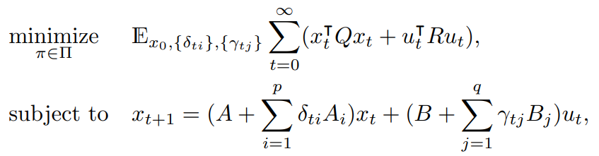
In this work, we consider the continuous-time analog of our previous work; i.e. we are interested in generating control commands that would render a continuous-time systems safe and enable it of satisfying its spatial and temporal requirements. Similarly, we consider stochastic linear systems affected by additive noise whose distribution belongs to the moment-based ambiguity set.
The continuous-time problem is more difficult.
Instead of having discrete control values to optimize over, we have to deal with stochastic integrals. But, stochastic integrals are mostly studied in the case of Gaussian noise. Thus, handling non-Gaussian cases is to some extent novel.
Finding an open-loop control over a horizon requires solving a constrained continuous-time optimization problem. Continuous-time optimal control is difficult itself (requires using Pontryagin’s maximum principle or solving the Hamilton-Jacobi-Bellman equation). In our problem we also have time-varying constraints.
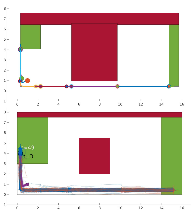
Top: tightened constraints seen by robot. Bottom: actual constraints. Robot avoids red regions (top and center) and has to alternate between visiting the left and right green regions
In our work, we provide a sufficient solution to the problem that consists of:
reformulating the dynamics to obtain deterministic risk-tightened dynamics
formulating a timed-transition continuous-time constrained problem and solving it by discretizing it while tightening our constraints to retain continuous-time guarantees
and finally stringing together solutions to the sequence of timed-transition problems.
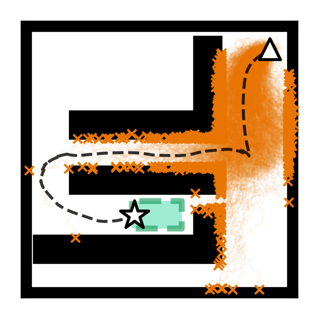
We propose a two-phase risk-averse architecture for controlling stochastic nonlinear robotic systems. RRT* is a high-level sampling-based planning algorithm that is appealing thanks to its asymptotic guarantees of completeness (if a solution exists, it will be found as the number of samples goes to infinity) and optimal (the solution will converge to the optimal value as the number of samples goes to infinity). However, such planners generally do not account for uncertainties while planning resulting in optimistic plans that are prone to failure under uncertainties. Notice how the figure on the left shows an RRT* tree that plans the robot trajectory from the triangle in the upper right corner to the green dashed rectangle passing through the narrow gap to the right of the obstacle. In pursuit of optimality, the plan gets dangerously close to the obstacles (black rectangles). To counter that, we present RANS-RRT*: Risk-Averse Nonlinear Steering RRT*, as an RRT* variant designed for nonlinear dynamics (solves a nonlinear program to steer between nodes) that accounts for risk by approximating the state distribution and applying a distributionally robust collision check to promote safe planning. The figure on the right depicts safety ellipses (yellow circles) at each node that must not collide with the obstacles. Notice how the plan thus avoids the aforementioned gap since it is deemed risky and instead approaches the goal region from the left side.
RRT*
RANS-RRT*
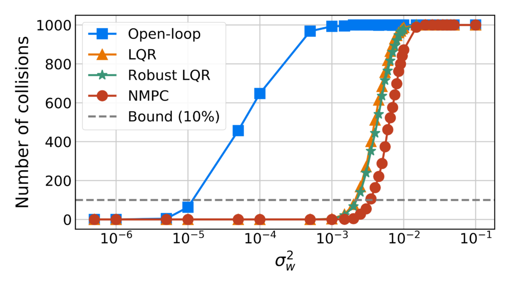
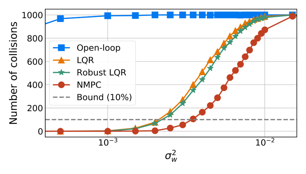
Having generated a risk-averse plan, the robot uses a low-level controller to track it. We compare three feedback controllers: linear quadratic regulator (LQR), LQR with robustness-promoting multiplicative noise terms (LQRm), and nonlinear model predictive control (NMPC) and the open-loop controller demonstrating the effectiveness of the the feedback controllers, and specifically the chosen NMPC tracker, under heavy-tailed Laplace process noise.
OL
LQR
LQRm
NMPC
We vary the size of the noise covariance from 0.0000005 to 0.1 and count the number of failures due to collisions out the 1000 Monte Carlo trials for each noise level. The results reveal NMPC’s superiority in tracking the trajectory more safely.
We propose a robust adaptive control algorithm that explicitly accounts for inherent non-asymptotic uncertainties arising from models estimated with finite, noisy data. The algorithm has three components: (1) a least-squares nominal model estimator; (2) a bootstrap resampling method that quantifies non-asymptotic variance of the nominal model estimate; and (3) a non-conventional robust control design method using an optimal linear quadratic regulator (LQR) with multiplicative noise. A key advantage of the proposed approach is that the system identification and robust control design procedures both use stochastic uncertainty representations, so that the actual inherent statistical estimation uncertainty directly aligns with the uncertainty the robust controller is being designed against. Numerical experiments show significant improvements over the certainty equivalent controller on both expected regret and measures of regret risk.
Keywords: Signal temporal logic, stochastic systems, constraint control, optimization
Summary
We present a framework for risk semantics on Signal Temporal Logic (STL) specifications for discrete-time linear dynamical systems with additive stochastic noise. Under our recursive risk semantics, risk constraints on STL formulas can be expressed in terms of risk constraints on atomic predicates which can be tightened into deterministic STL constraints on a related deterministic system. For affine predicates and the Distributionally Robust Value at Risk measure (DR-VaR), we show how the STL risk constraint is reformulated into a deterministic STL constraint. We demonstrate the framework using a Model Predictive Control (MPC) design.
Signal Temporal Logic (STL) has been a focus of recent control and robotics research because it provides expressive tools to formulate and reason about spatial and temporal system properties. A large fraction of this control synthesis under STL specifications literature primarily focuses on deterministic systems or stochastic systems with specific distributions (e.g. normal, bounded support, …) or incoherent risk metrics (e.g. chance constraint). However, practical systems are inherently stochastic and the disturbance may not always be know. Furthermore, it is compelling to use coherent risk metrics for robotics (where risk assessment follows four important risk axioms: monotonicity, translation invariance, positive homogeneity, and subadditivity). The need for frameworks that directly incorporate risk into the STL control synthesis problem is the primary motivation for our work.
Risk-Based STL
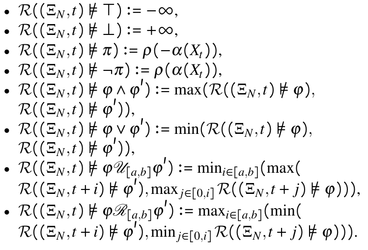
We use the STL grammar given by:
This grammar is know as the negation normal form (or positive normal form) and only includes negations at the atomic predicate level. The grammar builds formulas from the true boolean, an atomic predicate, the negation of an atomic predicate, the conjunction of two formulas, the disjunction of two formulas, the until temporal operator (satisfy the formula until the second is true), and the release operator. The atomic predicate is true if the system state applied to a predicate function is greater than zero and false if the latter is less than zero.
Since the system is stochastic, the system states form a stochastic process (rather than a deterministic run). This also make the predicate function with a stochastic state a random variable. We thus consider the risk of violating an STL formula and define the STL risk semantics.
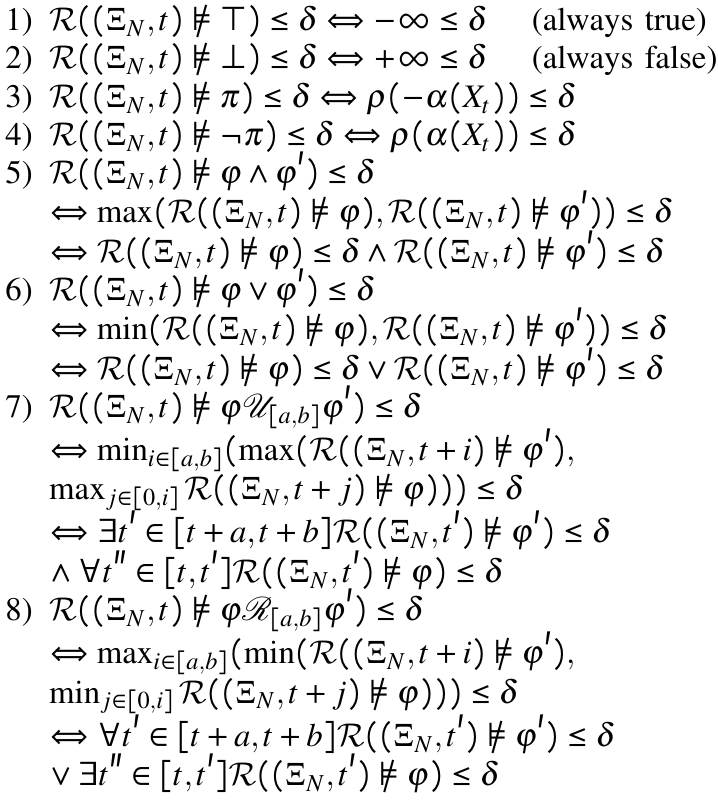
STL Formula Tightening
We first leverage the STL risk semantics to rewrite the STL risk constraint as a set of risk constraints on atomic predicates.
We can then reformulate the discrete-time stochastic system, assuming affine predicates, to find affine risk-tightened predicates. This uses the fact that any random variable can be divided into the sum of its mean and a 0-mean random variable. This also gives us a nominal system which is the expectation of the stochastic system.
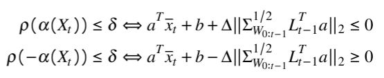
Reformulation for DR-VaR Risk Metric
Using the DR-VaR (distributionally robust value at risk) risk metric, Theorem 3.1 from “On distributionally robust chance-constrained linear programs” by Calafiore and El Ghaoui allows us to rewrite the risk-tightened constraints as deterministic affine inequalities.
Here, the overlined x term is the nominal state given by the expectation of the stochastic state, the Delta term in front of the norm is a constant that depends on the chosen risk-bound, the Sigma term is the covariance of the stochastic disturbance, the L term is a matrix based on the system dynamics (system A matrix), and the a,b terms come from the affine predicates.
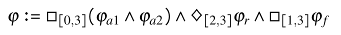
Numerical Experiments
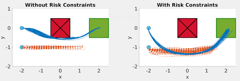
The experiment formula above, with appropriate predicates, encodes the following problem:
two agents ag1 and ag2 must always avoid a square obstacle centered at (0,0) with side length 1 over the time interval I1 = [0,3]
ag1 must eventually, over the time interval I2 = [2,3], reach a square goal region centered at (2,0)
ag1 and ag2 must maintain a maximum distance of 1 from each other over the time interval I3 = [1,3].
The simulation of 100 experiments yields the following results.
The left figure does not explicitly account for risk and thus collides with the obstacle with 84/100 runs failing to reach the goal because of the disturbance.
The right figure includes our proposed risk analysis with the tightened predicates. This keeps the trajectories sufficiently far from the obstacle and results in 98/100 runs reaching their goal safely.
We give novel characterizations of the uncertainty sets that arise in the robust linear quadratic regulator problem, develop Riccati equation-based solutions to optimal robust LQR problems over these sets, and give theoretical and empirical evidence that the resultant robust control law is a natural and computationally attractive alternative to the certainty-equivalent control law when the pair (A, B) is identified under l2-regularized linear least-squares.
Many thanks to Wouter Jongeneel and Dr. Peyman Esfahani at TU Delft for their collaboration on this work. Wouter has just finished his master’s thesis and is starting a PhD at EPFL under Daniel Kuhn January 2020 – congratulations!
We show that the linear quadratic regulator with multiplicative noise (LQRm) objective is gradient dominated, and thus applying policy gradient results in global convergence to the globally optimum control policy with polynomial dependence on problem parameters. The learned policy accounts for inherent parametric uncertainty in system dynamics and thus improves stability robustness. Results are provided both in the model-known and model-unknown settings where samples of system trajectories are used to estimate policy gradients.
Policy gradient is a general algorithm from reinforcement learning; see Ben Recht’s gentle introduction. At a high level, it is simply the application of (stochastic) gradient descent to the parameters of a parametric control policy. Although traditional reinforcement learning treats the tabular setting with discrete state and action spaces, most real-world control problems deal with systems that have continuous state and action spaces. Luckily, policy gradient works much the same way in this setting.
In this post we walk through some of the key points from our paper; see the full text for more details and variable definitions.
Setting: LQR with multiplicative noise
We consider the following infinite-horizon stochastic optimal control problem with an objective quadratic in the state and input with stochastic dynamics with multiplicative noises (LQRm problem). Expectation is with respect to the initial state and the multiplicative noise.
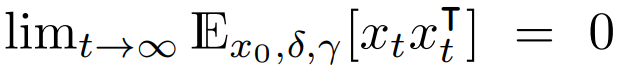
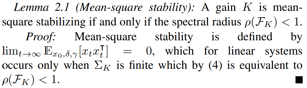
Any solution to this problem must be stabilizing, however in the context of stochastic systems we must deal with a stronger form of stability known as mean-square stability which requires not only that the expected state return to the origin over time, but also that the (auto)covariance of the state decrease to zero over time:
Mean-square stability:
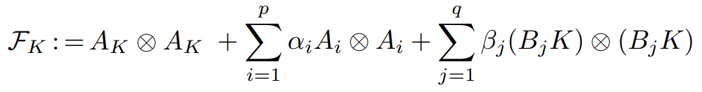
Mean-square stability can be further characterized in terms of the vectorized state covariance dynamics operator
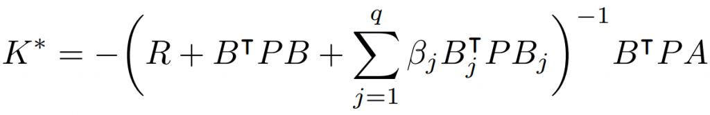
The LQRm problem is special since it, like the deterministic LQR problem, admits a simple solution which is computable from a Riccati equation, specifically this one:
However, unlike the LQR problem with additive noise, the multiplicative noises change the optimal gain matrix relative to the deterministic case. In particular, the multiplicative noise can be used as a proxy for uncertainty in the model parameters of a deterministic linear model.
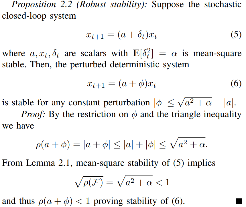
Motivation: robust stability
A key issue in control design is robustness i.e. ensuring stability in the presence of model parameter uncertainty. The following example motivates how stochastic multiplicative noise ensures deterministic robustness.
Although this is a simple example, it demonstrates that the robustness margin increases monotonically with the multiplicative noise variance. We also see that when α = 0 the bound collapses so that no robustness is guaranteed, i.e., when |a| → 1. This result can be extended to multiple states, inputs, and noise directions, but the resulting conditions become considerably more complex.
Case of known dynamics
We already saw that we can solve the optimal control problem exactly (up to a Riccati equation), so what else is there to study? We ultimately care about the case when dynamics are unknown (e.g. as in adaptive control or system identification) which can be handled by policy gradient.
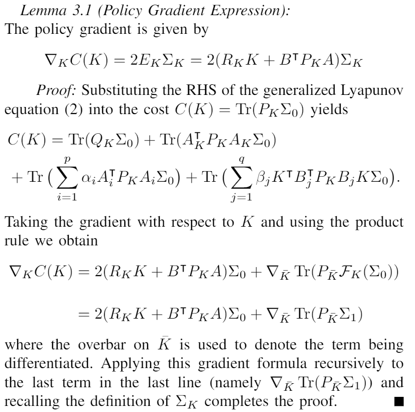
To begin we see how policy gradient works when the dynamics are fully known, in which case the policy gradient can be evaluated analytically in terms of the dynamics:
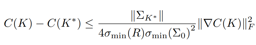
With this expression, we can prove the key result that the LQRm objective is gradient dominated in the control gain matrix K:
This (along with Lipschitz continuity) immediately implies that (policy) gradient descent with an appropriate constant step size will converge to the global minimum, i.e. the same solution found by solving a Riccati equation, at a linear (geometric) rate from any initial point. For those familiar with convex optimization, gradient domination bears some similarities to the more restrictive strong convexity condition, which essentially puts a lower bound on the curvature of the function, thus ensuring gradient descent makes sufficient progress at each step anywhere on the function. See Theorem 1 of this paper for an extremely short proof of convergence under the gradient domination (Polyak-Lojasiewicz) condition.
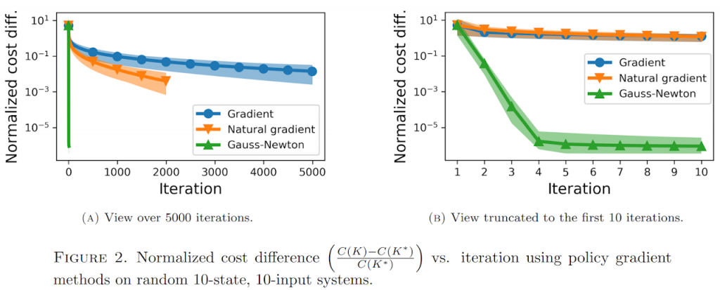
The bulk of the technical work that follows goes towards bounding the Lipschitz constant, and thus the step size and convergence rate. We also analyze the natural policy gradient and “Gauss-Newton” steps in parallel to Fazel et al. – these steps give faster convergence than vanilla policy gradient but require more information. Note that “Gauss-Newton” step with a stepsize of 1/2 is exactly the policy iteration algorithm (another model-free RL technique) first proven to converge for standard LQR in the case of known dynamics in continuous-time by Kleinman in 1968 and in discrete-time by Hewer in 1971 and in the case of unknown dynamics by Bradtke, Ydstie, and Barto at the 1994 ACC. Note that many authors from the 1960s and 1970s did not frame their results under the modern dynamic programming/reinforcement learning labels of “policy iteration” or “Q-learning” but rather as iterative solutions of Riccati equations.
Case of unknown dynamics
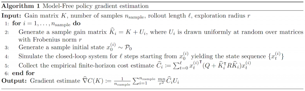
When the dynamics are unknown, the (policy) gradient must be obtained empirically via estimation from sample trajectories. We use the following algorithm to do this:
In this case, we use tools from high-dimensional statistics known as concentration bounds to ensure that with high probability the error between the estimated and true gradients is smaller than a threshold. The threshold is chosen small enough that gradient descent with the same step size as in the case of exact gradients provably converges.
Numerical experiments
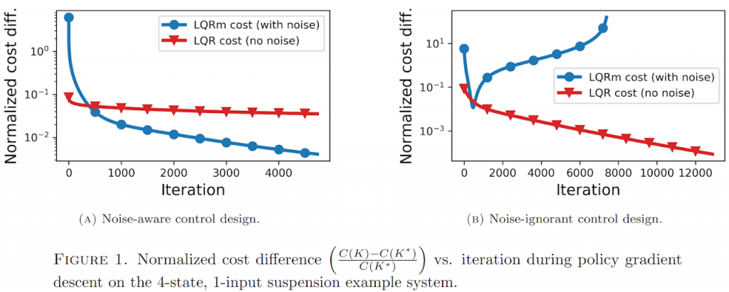
We validated policy gradient in the case of known dynamics – this is much faster to simulate than the case of unknown dynamics due to the large number of samples required to estimate the policy gradient accurately.
The first example shows policy gradient working on a suspension system with 2 masses (4 states) and a single input. To demonstrate the peril of failing to account for multiplicative noise when it truly exists, we ran policy gradient both (a) accounting for and (b) ignoring the multiplicative noise. The blue curves show the control evaluated on the LQR cost with multiplicative noise while the red curves show the control evaluated on the LQR cost without multiplicative noise. When the noise is ignored, the control destabilized the truly noisy system in mean-square. When noise is assumed, the control achieves lower performance on the truly noiseless system, but does not and cannot destabilize it.
The second example shows policy gradient and its faster cousins applied on a random 10-state, 10-input system. With more iterations, the global optimum is more closely approximated.
Opinions & take-aways
Although the techniques used in this work and Fazel et al. represent a novel synthesis of tools from various mathematical fields, simpler/shorter proofs would help reduce barriers-to-entry for controls researchers unfamiliar with the finer points of reinforcement learning and statistics.
Convergence results were shown, but sample efficiency is still a major concern. Model-based techniques have been shown to be significantly more efficient for learning to control linear systems. This is somewhat expected since a linear dynamics model is the simplest possible; model-free techniques may be competitive when the dynamics are highly nonlinear and difficult to model based solely on data.
Related work
We envision multiplicative noise as a modeling framework for ensuring robustness; see older work from Bernstein which informs this notion. Perhaps the best known framework for robustness in multivariate state space control is H-infinity control. Applying policy gradient to the dynamic game formulation of this framework has received attention lately as well; see positive results in the two-player setting and negative results in the many-player setting.