Control Design for Risk-Based Signal Temporal Logic Specifications

Sleiman Safaoui, Lars Lindemann, Dimos V Dimarogonas, Iman Shames, Tyler H Summers, IEEE L-CSS/CDC 2020

Keywords: Signal temporal logic, stochastic systems, constraint control, optimization

Summary

We present a framework for risk semantics on Signal Temporal Logic (STL) specifications for discrete-time linear dynamical systems with additive stochastic noise. Under our recursive risk semantics, risk constraints on STL formulas can be expressed in terms of risk constraints on atomic predicates which can be tightened into deterministic STL constraints on a related deterministic system. For affine predicates and the Distributionally Robust Value at Risk measure (DR-VaR), we show how the STL risk constraint is reformulated into a deterministic STL constraint. We demonstrate the framework using a Model Predictive Control (MPC) design.

Get paper on IEEE Xplore or arXiv.

Overview

Signal Temporal Logic (STL) has been a focus of recent control and robotics research because it provides expressive tools to formulate and reason about spatial and temporal system properties. A large fraction of this control synthesis under STL specifications literature primarily focuses on deterministic systems or stochastic systems with specific distributions (e.g. normal, bounded support, …) or incoherent risk metrics (e.g. chance constraint). However, practical systems are inherently stochastic and the disturbance may not always be know. Furthermore, it is compelling to use coherent risk metrics for robotics (where risk assessment follows four important risk axioms: monotonicity, translation invariance, positive homogeneity, and subadditivity). The need for frameworks that directly incorporate risk into the STL control synthesis problem is the primary motivation for our work.

Risk-Based STL

We use the STL grammar given by:

This grammar is know as the negation normal form (or positive normal form) and only includes negations at the atomic predicate level. The grammar builds formulas from the true boolean, an atomic predicate, the negation of an atomic predicate, the conjunction of two formulas, the disjunction of two formulas, the until temporal operator (satisfy the formula until the second is true), and the release operator. The atomic predicate is true if the system state applied to a predicate function is greater than zero and false if the latter is less than zero.

Since the system is stochastic, the system states form a stochastic process (rather than a deterministic run). This also make the predicate function with a stochastic state a random variable. We thus consider the risk of violating an STL formula and define the STL risk semantics.

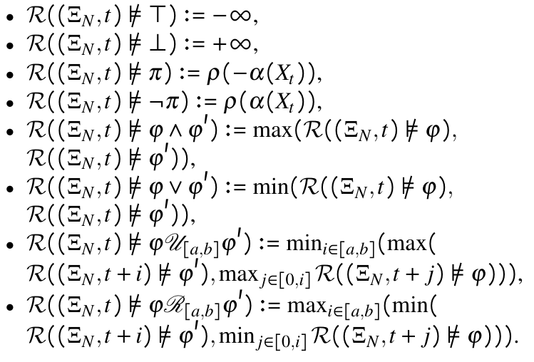
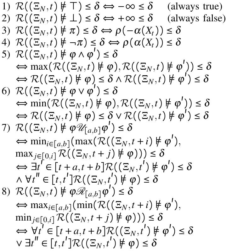
STL Formula Tightening

We first leverage the STL risk semantics to rewrite the STL risk constraint as a set of risk constraints on atomic predicates.

We can then reformulate the discrete-time stochastic system, assuming affine predicates, to find affine risk-tightened predicates. This uses the fact that any random variable can be divided into the sum of its mean and a 0-mean random variable. This also gives us a nominal system which is the expectation of the stochastic system.

Reformulation for DR-VaR Risk Metric

Using the DR-VaR (distributionally robust value at risk) risk metric, Theorem 3.1 from “On distributionally robust chance-constrained linear programs” by Calafiore and El Ghaoui allows us to rewrite the risk-tightened constraints as deterministic affine inequalities.

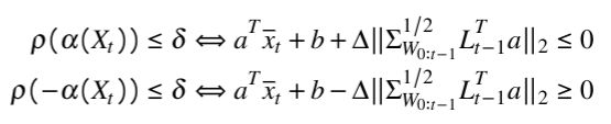
Here, the overlined x term is the nominal state given by the expectation of the stochastic state, the Delta term in front of the norm is a constant that depends on the chosen risk-bound, the Sigma term is the covariance of the stochastic disturbance, the L term is a matrix based on the system dynamics (system A matrix), and the a,b terms come from the affine predicates.

Numerical Experiments

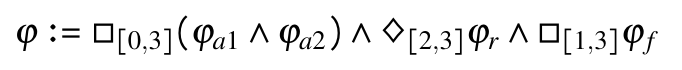
The experiment formula above, with appropriate predicates, encodes the following problem:

two agents ag1 and ag2 must always avoid a square obstacle centered at (0,0) with side length 1 over the time interval I1 = [0,3]
ag1 must eventually, over the time interval I2 = [2,3], reach a square goal region centered at (2,0)
ag1 and ag2 must maintain a maximum distance of 1 from each other over the time interval I3 = [1,3].

The simulation of 100 experiments yields the following results.

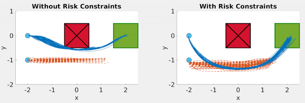
The left figure does not explicitly account for risk and thus collides with the obstacle with 84/100 runs failing to reach the goal because of the disturbance.

The right figure includes our proposed risk analysis with the tightened predicates. This keeps the trajectories sufficiently far from the obstacle and results in 98/100 runs reaching their goal safely.