Work by Hamed Karimi, Julie Nutini, and Mark Schmidt, ECML PKDD 2016

Keywords: Nonconvex, optimization, Polyak-Lojasiewicz inequality, gradient domination, convergence, global

Summary

The authors re-explore the Polyak-Lojasiewicz inequality first analyzed by Polyak in 1963 by deriving convergence results under various descent methods for various modern machine learning tasks and establishing equivalences and sufficiency-necessity relationships with several other nonconvex function classes. A highlight of the paper is a beautifully simple proof of linear convergence using gradient descent on PL functions, which we walk through in our discussion.

Read the paper on arXiv here.

Convergence of gradient descent under the Polyak-Lojasiewicz inequality

This proof is extremely short and simple, requiring only a few assumptions and a basic mathematical background. It is strange that it is as universally known as the theory related to convex optimization.

Relating to the theory of Lyapunov stability for nonlinear systems, the PL inequality essentially means that the function value itself is a valid Lyapunov function for exponential stability of the global minimum under the nonlinear gradient descent dynamics.

Lieven Vandenberghe’s lecture notes for the case of strongly convex functions are an excellent supplement.

The setting we consider is that of minimizing a function f(x).

Lipschitz continuity

A function is Lipschitz continuous with constant L if

Likewise the gradient (first derivative) of a function is Lipschitz continuous with constant L if

For the next steps we follow slide 1.13 of Lieven Vandenberghe’s lecture notes.

Recall the Cauchy-Schwarz inequality

Applying the Cauchy-Schwartz inequality to the Lipschitz gradient condition gives

Define the function g(t) as

If the domain of f is convex, then g(t) is well-defined for all t in [0, 1].

Using the definition of g(t), the chain rule of multivariate calculus, and the previous inequality we have

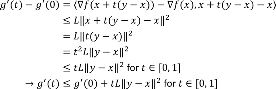
Using the definition of g(t) we can rewrite f(y) in terms of an integral by using the fundamental theorem of calculus

Integrating the second term from 0 to t and using the previous inequality and the derivative of g(t) we obtain

Substituting back into the expression for f(y) we obtain the quadratic upper bound

The Polyak-Lojasiewicz inequality

A function is said to satisfy the Polyak-Lojasiewicz inequality if the following condition holds:

where f* is the minimum function value.

This means that the norm of the gradient grows at least as fast as a quadratic as the function value moves away from the optimal function value.

Additionally, this implies that every stationary point of f(x) is a global minimum.

Gradient descent

The gradient descent update simply takes a step in the direction of the negative gradient:

We are now ready to prove convergence of gradient descent under the PL inequality i.e. Theorem 1 of Karimi et al.

Rearranging the gradient descent update gives the difference

Using the gradient descent update rule in the quadratic upper bound condition (from Lipschitz continuity of the gradient) we obtain

If the stepsize is chosen so that the coefficient on the righthand side is negative, then using the Polyak-Lojasiewicz inequality gives

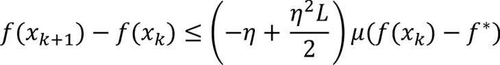
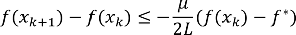
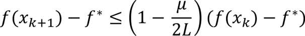
The range of permissible stepsizes is [0, 2/L] with the best rate achieved with a stepsize of 1/L. Under this choice, we obtain

Adding f(x_k) – f* to both sides gives

Dividing by f(x_k) – f* gives the linear (geometric) convergence rate

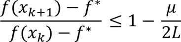
This shows that the difference between the current function value and the minimum decreases at least as fast as a geometric series with a rate determined by the ratio of the PL and Lipschitz constants.

Why would control systems researchers care about this?

The Polyak-Lojasiewicz inequality is key to analysis of convergence of policy gradient for LQR and LQR with multiplicative noise.